library(momentuHMM)
library(tidyverse)
source(here::here("R/dives.R"))

#read in dive type data (done manually)
dive_type <- read_csv(here::here("data/manual-dive-type.csv")) %>%
  select(-c(AcousticsUsed, Notes)) %>%
  mutate(ID = 1,
         Benthic_Pelagic_int = unclass(factor(Benthic_Pelagic,
                                              levels = c("Benthic",
                                                         "Pelagic"))),
         Rest_Forage_Travel_int = unclass(factor(Rest_Forage_Travel,
                                                 levels = c("Rest",
                                                            "Forage",
                                                            "Travel"))))

dive_prepped <- prepData(data = dive_type,
coordNames = NULL)Dive behavior
Use momentuHMM to fit a Hidden Markov Model to the dive data.
First, read in and prep the data.
Fit the HMM.
##### 3 state model #####

# Define initial parameters
nbStates <- 3  # number of hidden states

# order of initial states is Rest, Forage, Travel
one <- 0.99
zero <- function(k) (1 - one) / (k - 1)
cat_pars <- list(
  Rest_Forage_Travel_int = c(
    # P(R) for states R, F, T
    one, zero(3), zero(3),
    # P(F) for states R, F, T
    zero(3), one, zero(3)
    # P(T) implied
  )
)

# Fit HMM
hmm_fit3 <- fitHMM(data = dive_prepped,
                   nbStates = nbStates,
                   dist = list(Rest_Forage_Travel_int = "cat3"),
                   Par0 = cat_pars,
                   stateNames = c("Rest", "Forage", "Travel"))
hmm_fit3
Value of the maximum log-likelihood: -1180.064
Rest_Forage_Travel_int parameters:
----------------------------------
Rest Forage Travel
prob1 0.95431278 8.741234e-10 0.004918582
prob2 0.02029864 9.818222e-01 0.357142234
Regression coeffs for the transition probabilities:
---------------------------------------------------
1 -> 2 1 -> 3 2 -> 1 2 -> 3 3 -> 1 3 -> 2
(Intercept) -1.478254 -3.58744 -2.956297 -3.915859 -3.562337 -3.564553
Transition probability matrix:
------------------------------
Rest Forage Travel
Rest 0.79636570 0.18159960 0.02203470
Forage 0.04852085 0.93289273 0.01858642
Travel 0.02685049 0.02679107 0.94635844
Initial distribution:
---------------------
Rest Forage Travel
1.546404e-06 8.591688e-09 9.999984e-01 Now fitting the 3 state HMM with SW presence/absence in the dive as an environmental covariate.
recording <- read_rds(here::here("output/recording_calib.rds"))
dive_summ <- read_rds(here::here("output/processed_dive_summaries.rds"))

###assign dive ids
find_next <- function(x, y) {
  # Find the index of the next value in y following x
  approx(y,
         seq_along(y),
         method = "constant",
         f = 1,
         rule = 2,
         xout = x)$y
}

clicks_by_dive <- read_csv(here::here("data/sw/clicks_by_dive.csv")) %>%
  #trying to connect recording with the correct dive id
  mutate(end_calib = recording$end_calib[-nrow(recording)],
         dive_id = dive_summ$dive_id[find_next(end_calib, dive_summ$end)],
         sw_yn = sw_yn == "y") %>%
  select(-c(clickmanual_complete, buzz, notes)) %>%
  left_join(select(dive_type, dive_id, Rest_Forage_Travel_int, ID),
            by = "dive_id")

dive_sw_prepped <- prepData(clicks_by_dive,
                            coordNames = NULL)

# Fit HMM w sw as a covariate
hmm_fit3_sw <- fitHMM(data = dive_sw_prepped,
                      nbStates = nbStates,
                      formula = ~ sw_yn,
                      dist = list(Rest_Forage_Travel_int = "cat3"),
                      Par0 = cat_pars,
                      fixPar = list(beta = matrix(
                        c(NA, NA, NA, NA, NA, NA,
                          NA,  0, NA,  0,  0,  0),
                        nrow = 2, byrow = TRUE
                      )),
                      stateNames = c("Rest", "Forage", "Travel"))

hmm_fit3_sw
Value of the maximum log-likelihood: -1170.661
Rest_Forage_Travel_int parameters:
----------------------------------
Rest Forage Travel
prob1 0.96402740 1.043392e-10 0.005099622
prob2 0.02051549 9.802998e-01 0.325123667
Regression coeffs for the transition probabilities:
---------------------------------------------------
1 -> 2 1 -> 3 2 -> 1 2 -> 3 3 -> 1 3 -> 2
(Intercept) -1.4637675 -3.589279 -2.957103 -3.860541 -3.537286 -3.347382
sw_ynTRUE -0.1310757 0.000000 -0.161613 0.000000 0.000000 0.000000
Transition probability matrix (based on mean covariate values):
---------------------------------------------------------------
Rest Forage Travel
Rest 0.79750122 0.18047320 0.02202558
Forage 0.04719010 0.93316069 0.01964921
Travel 0.02733538 0.03305213 0.93961249
Initial distribution:
---------------------
Rest Forage Travel
2.844813e-07 9.866245e-10 9.999997e-01 ci <- CIbeta(hmm_fit3_sw, alpha = 0.05)
ci$beta # coefficients, SEs, and 95% CIs for each transition$est
1 -> 2 1 -> 3 2 -> 1 2 -> 3 3 -> 1 3 -> 2
(Intercept) -1.4637675 -3.589279 -2.957103 -3.860541 -3.537286 -3.347382
sw_ynTRUE -0.1310757 0.000000 -0.161613 0.000000 0.000000 0.000000
$se
1 -> 2 1 -> 3 2 -> 1 2 -> 3 3 -> 1 3 -> 2
(Intercept) 0.1582089 0.4356679 0.1588249 0.2862058 0.3119624 0.4329451
sw_ynTRUE 0.3823005 0.0000000 0.3599052 0.0000000 0.0000000 0.0000000
$lower
1 -> 2 1 -> 3 2 -> 1 2 -> 3 3 -> 1 3 -> 2
(Intercept) -1.4736883 -3.616598 -2.9670626 -3.878488 -3.556848 -3.37453
sw_ynTRUE -0.1550486 0.000000 -0.1841815 0.000000 0.000000 0.00000
$upper
1 -> 2 1 -> 3 2 -> 1 2 -> 3 3 -> 1 3 -> 2
(Intercept) -1.4538467 -3.561959 -2.9471438 -3.842593 -3.517724 -3.320233
sw_ynTRUE -0.1071029 0.000000 -0.1390445 0.000000 0.000000 0.000000#some NAs for transitions where probabilities were constrained near 0.
beta_table <- bind_cols(
as.data.frame.table(ci$beta$est,
responseName = "est"),
as.data.frame.table(ci$beta$se,
responseName = "se") %>%
select(se),
as.data.frame.table(ci$beta$lower,
responseName = "lower") %>%
select(lower),
as.data.frame.table(ci$beta$upper,
responseName = "upper") %>%
select(upper)
) %>%
rename(parameter = Var1, transition = Var2)
library(kableExtra)
beta_table %>%
mutate(across(where(is.numeric), ~ round(.x, 3))) %>% #round to 3 places
kable(col.names = c("Parameter", "Transition", "Estimate", "SE", "Lower 95%", "Upper 95%"),
caption = "Beta coefficients") %>%
kable_styling(bootstrap_options = c("striped", "hover")) | Parameter | Transition | Estimate | SE | Lower 95% | Upper 95% |
|---|---|---|---|---|---|
| (Intercept) | 1 -> 2 | -1.464 | 0.158 | -1.474 | -1.454 |
| sw_ynTRUE | 1 -> 2 | -0.131 | 0.382 | -0.155 | -0.107 |
| (Intercept) | 1 -> 3 | -3.589 | 0.436 | -3.617 | -3.562 |
| sw_ynTRUE | 1 -> 3 | 0.000 | 0.000 | 0.000 | 0.000 |
| (Intercept) | 2 -> 1 | -2.957 | 0.159 | -2.967 | -2.947 |
| sw_ynTRUE | 2 -> 1 | -0.162 | 0.360 | -0.184 | -0.139 |
| (Intercept) | 2 -> 3 | -3.861 | 0.286 | -3.878 | -3.843 |
| sw_ynTRUE | 2 -> 3 | 0.000 | 0.000 | 0.000 | 0.000 |
| (Intercept) | 3 -> 1 | -3.537 | 0.312 | -3.557 | -3.518 |
| sw_ynTRUE | 3 -> 1 | 0.000 | 0.000 | 0.000 | 0.000 |
| (Intercept) | 3 -> 2 | -3.347 | 0.433 | -3.375 | -3.320 |
| sw_ynTRUE | 3 -> 2 | 0.000 | 0.000 | 0.000 | 0.000 |
If the CI excludes zero, the covariate effect on that transition is significant.
# dive_sw_prepped %>%
#   mutate(state = Rest_Forage_Travel_int,
#          next_state = lead(Rest_Forage_Travel_int)) %>%
#   count(state, next_state, sw_yn) %>%
#   drop_na(next_state) %>%
#   group_by(state, sw_yn) %>%
#   mutate(freq = n / sum(n)) %>%
#   ungroup() %>%
#   arrange(state, sw_yn, next_state) %>%
#   filter(next_state == 2) %>%
#   view()

p <- ggplot(dive_sw_prepped, aes(start_time, Rest_Forage_Travel_int)) +
  geom_line() +
  geom_point(aes(color = sw_yn, group = dive_id))
plotly::ggplotly(p, dynamicTicks = TRUE)
Are there differences in the dive characteristics when sw are present?
dive_sw_prepped %>%
  group_by(Rest_Forage_Travel_int, sw_yn) %>%
  summarize(dur_mean = mean(duration_min),
            dur_sd = sd(duration_min),
            .groups = "drop") %>%
  mutate(sw_yn = ifelse(sw_yn, "sw_present", "sw_absent")) %>%
  pivot_wider(names_from = sw_yn, values_from = c(dur_mean, dur_sd))
# A tibble: 3 × 5
Rest_Forage_Travel_int dur_mean_sw_absent dur_mean_sw_present dur_sd_sw_absent
<int> <dbl> <dbl> <dbl>
1 1 21.5 22.9 4.61
2 2 19.7 22.2 3.59
3 3 18.5 19.7 4.36
# ℹ 1 more variable: dur_sd_sw_present <dbl>library(nlme)
# Limit analysis to foraging dives 10+ minutes long
foraging_dives <- dive_sw_prepped %>%
filter(duration_min >= 10,
Rest_Forage_Travel_int == 2) %>%
mutate(hours_elapsed = as.numeric(start_time - start_time[1], unit = "hours"))
dive_dur <- gls(duration_min ~ sw_yn,
foraging_dives,
correlation = corCAR1(form = ~ hours_elapsed))
summary(dive_dur)Generalized least squares fit by REML
Model: duration_min ~ sw_yn
Data: foraging_dives
AIC BIC logLik
6366.22 6387.231 -3179.11
Correlation Structure: Continuous AR(1)
Formula: ~hours_elapsed
Parameter estimate(s):
Phi
0.4381037
Coefficients:
Value Std.Error t-value p-value
(Intercept) 20.216678 0.1913875 105.63219 0
sw_ynTRUE 1.658956 0.3821592 4.34101 0
Correlation:
(Intr)
sw_ynTRUE -0.369
Standardized residuals:
Min Q1 Med Q3 Max
-3.5852686 -0.5807263 -0.1023656 0.4796796 6.2365335
Residual standard error: 3.158936
Degrees of freedom: 1414 total; 1412 residual# binned ACF for each model
irreg_acf <- function(mod) {
r <- residuals(mod, type = "normalized")
t <- foraging_dives$hours_elapsed
pairs <- expand_grid(i = seq_along(r), j = seq_along(r)) %>%
filter(j > i) %>%
mutate(lag = abs(t[i] - t[j]),
prod = r[i] * r[j]) %>%
filter(lag <= 24)
bin_width = 0.5
pairs %>%
mutate(lag_bin = floor(lag / bin_width) * bin_width + bin_width / 2) %>%
group_by(lag_bin) %>%
summarize(acf = mean(prod), n = n()) %>%
slice(-n()) %>%
ggplot(aes(lag_bin, acf)) +
geom_hline(yintercept = 0 ) +
geom_hline(yintercept = c(-1.96, 1.96) / sqrt(length(t)),
linetype = "dashed", color = "blue") +
geom_col()
}
irreg_acf(dive_dur)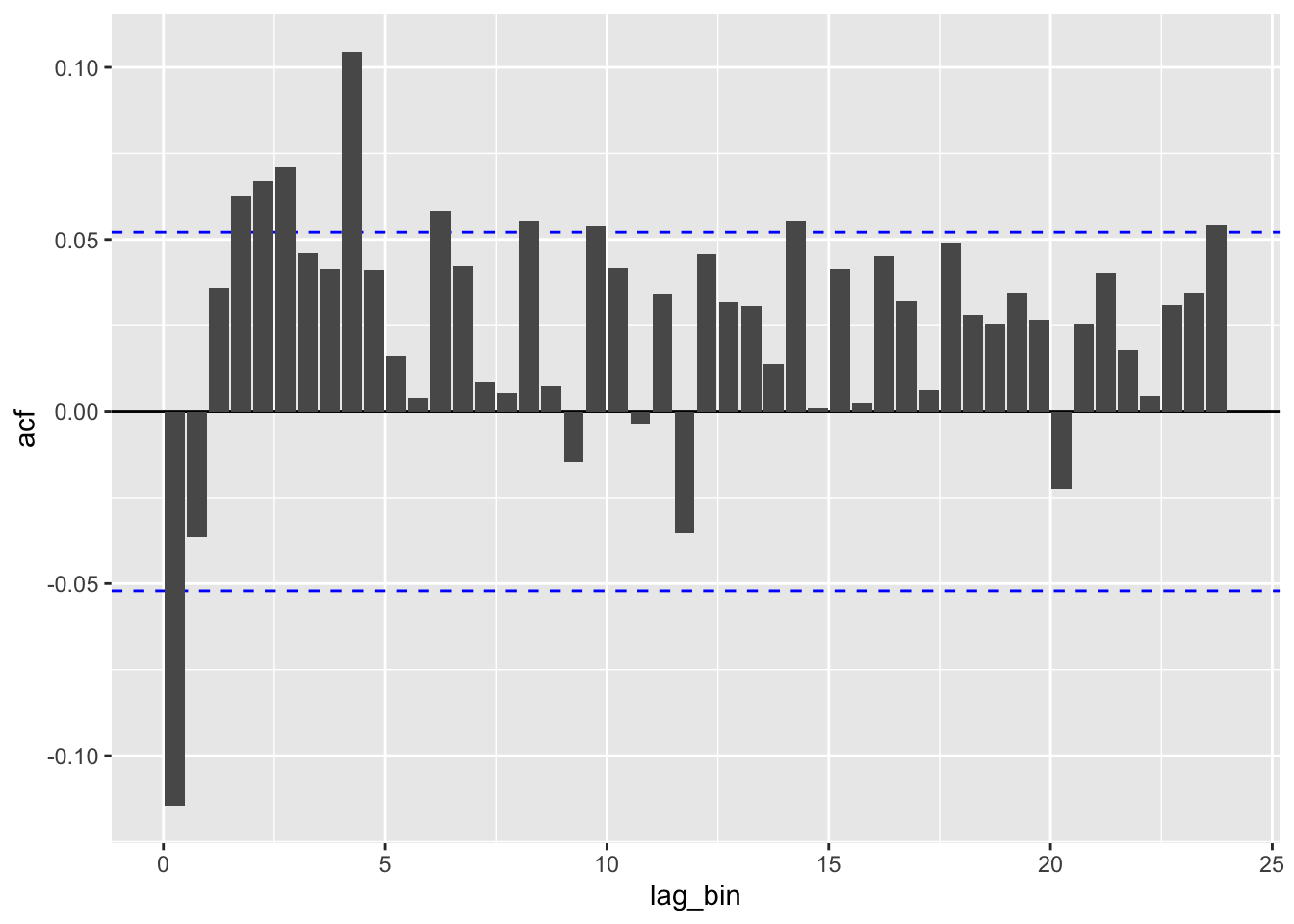
Dive duration is on average 1-2 mins longer when sperm whales are present.