Fine scale

First, read in the dive data and split into individual dives.

library(tidyverse)
library(zoo)
library(gridExtra)
source(here::here("R/dives.R"))

depth <- read_csv(here::here("data/23A1302/out-Archive.csv"), show_col_types = FALSE) %>%
  drop_na(Depth) %>% 
  mutate(Date = as.POSIXct(Time, format = "%H:%M:%S %d-%b-%Y", tz = "UTC")) %>% 
  rename(no_zoc_depth = Depth,
         Depth = `Corrected Depth`)

dives <- get_dives(depth, 5, 80)

Next, load in the acoustic data. We have two kinds of acoustic data: manual annotations of sperm whale bouts, and triton-detected sperm whale clicks (aka, TPWS). We want to compare them and make sure they look similar.

to-do: update the manual annotations, they are newly validated.

source(here::here("R/broad_funcs.R"))

#sw_comb_bouts has just sperm whales, and all nearby bouts are combined. 

manual <- read.csv(here::here("data/sw_comb_bouts.csv")) 

#convert times to POSIXct and add boutID
manual <- manual %>% 
  mutate(start = ymd_hms(start, tz = "UTC"), 
         end = ymd_hms(end, tz = "UTC"), 
         bout = row_number())

window_hr <- 12

sw_manual <- tibble(date = seq(first(manual$start), last(manual$end), by = window_hr * 3600)) %>% 
  mutate(SW = map_dbl(date, \(d) sum_odon_exposure(data = manual, d)))

#read in each triton-found click with RL measurement (MPP, measured in dB)
tpws <- read.csv(here::here("data/sw/tpws.csv"), header = FALSE) %>% 
  rename(clicktime = V1, MPP = V2)

#convert the matlab dates to UTC
tpws <- tpws %>% 
  mutate(clicktime = as.POSIXct((clicktime - 719529) * 86400, 
                      origin = "1970-01-01", 
                      tz = "UTC"))

ggplot(tpws, aes(clicktime)) + 
  geom_histogram(color = "white", fill = "gray") +
  geom_line(data = sw_manual, aes(date, SW * 800), color = "hotpink") +
  theme_bw()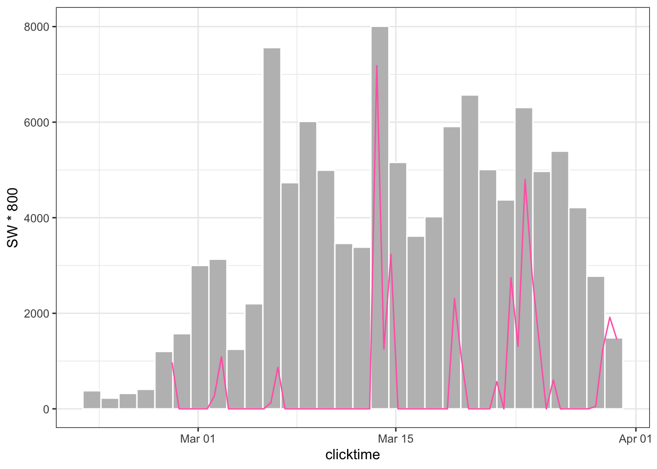

Cutting tpws to the manual annotations, but show 5 hours of tpws + dives on either side.

#filter tpws to only include times in the validated manual annotations
tpws_val <- manual %>% 
  mutate(data = map2(start - hours(5), end + hours(5), ~ {
    tpws %>% 
      filter(clicktime >= .x & clicktime <= .y)
  })) %>% 
  unnest(data) %>% 
  select(bout, start, end, clicktime, MPP)

# #choose window in minutes, then create columns for the window in the data frame
window_min <- 5
tpws_val <- tpws_val %>%
  mutate(time_elapsed = difftime(clicktime, start, units = "secs"),
         window = floor(as.numeric(time_elapsed / (window_min * 60))),
         win_start = start + seconds(window * window_min * 60))

# #calculate the average received level for each window
avg_Rl <- tpws_val %>%
  group_by(bout, win_start) %>%
  summarize(mean_MPP = mean(MPP, na.rm = TRUE),
            clicks_per_bin = n(),
            .groups = "drop")

#put the window average RLs into the tpws data frame
tpws_full <- tpws_val %>% 
  inner_join(avg_Rl, by = "win_start")

#get the dive starts so that we can also calcualte mean RL for each dive
dive_starts <- dives %>% 
  group_by(dive_id) %>% 
  slice(1) %>% 
  ungroup() %>% 
  select(dive_id, Date)

#add a column to the twps dataframe which has the associated dive ID for each detection
tpws_full$dive_id <- findInterval(tpws_full$clicktime, dive_starts$Date)

Calculating when the device was NOT recording audio.

source(here::here("R/non_recording.R"))

#wav_timestamps.csv is the output of the function get_wav_timestamps.R. 
recording <- read.csv(here::here("data/wav_timestamps.csv")) %>% 
                        mutate(start = ymd_hms(start_time, tz = "UTC"),
                               end = ymd_hms(end_time, tz = "UTC")) %>% 
                        drop_na(end)

non_recording <- calculate_non_recording(recording)

Plotting the received level vs. time on top, with the dive record underneath.

source(here::here("R/fine_plots.R"))

#make the plots
bout_plots <- map(1:nrow(manual), 
                   ~make_bout_plot(.x, tpws_full, depth, non_recording, manual)) 

bout_plots

[[1]]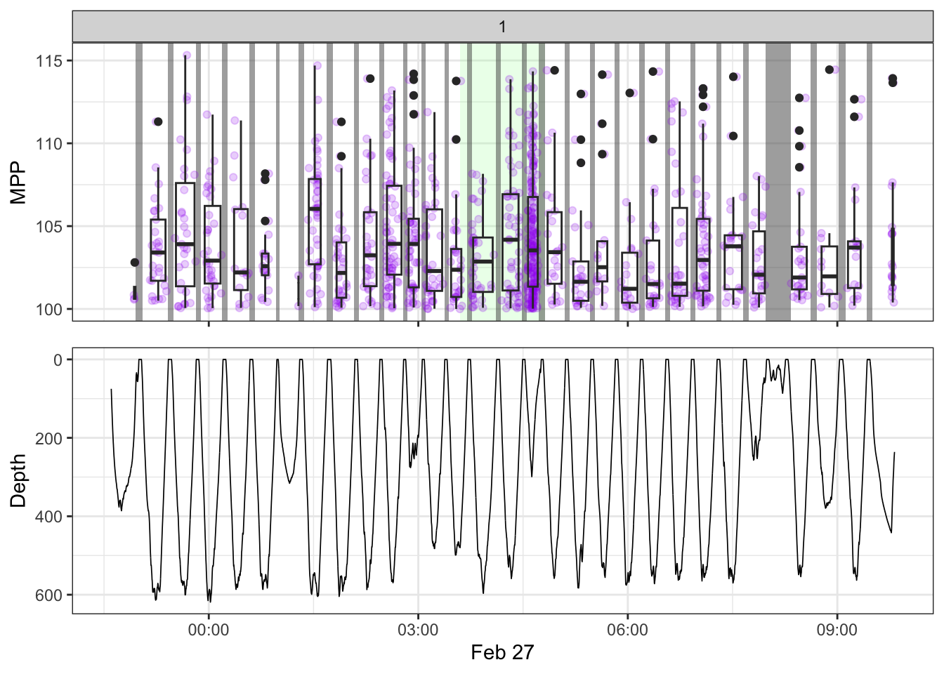

[[2]]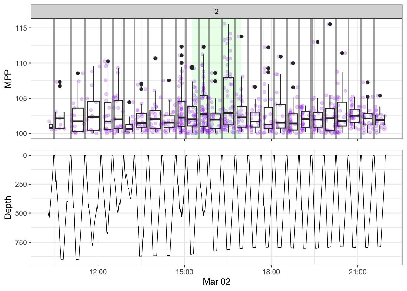

[[3]]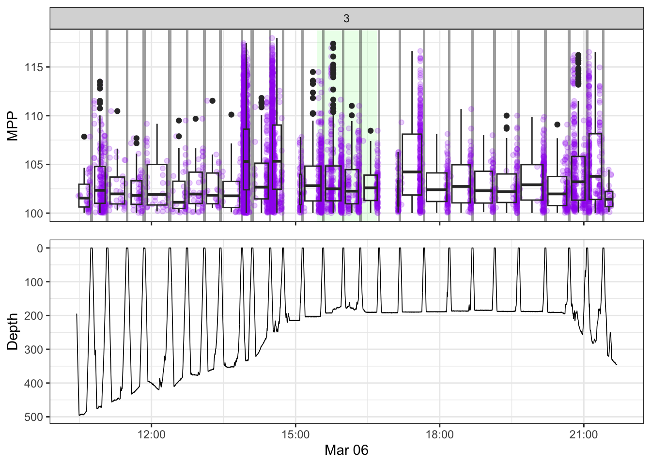

[[4]]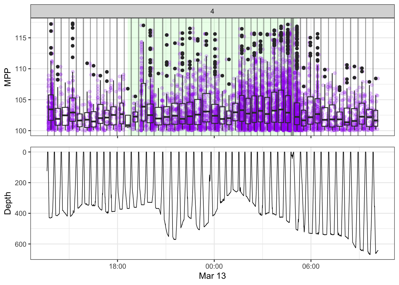

[[5]]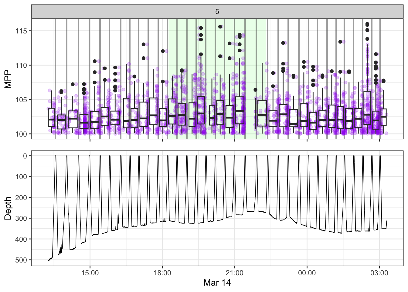

[[6]]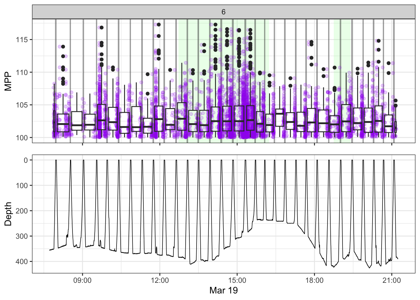

[[7]]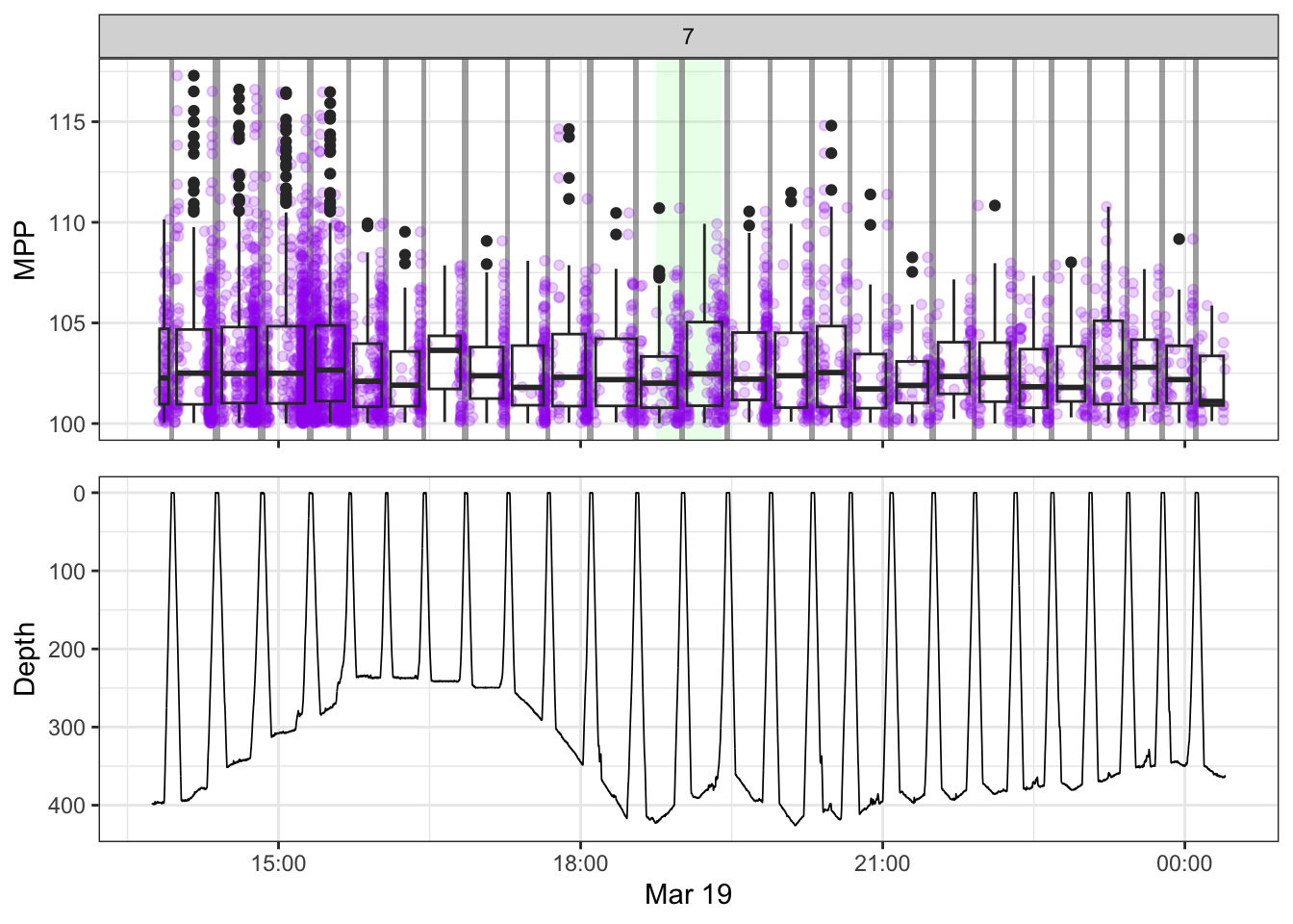

[[8]]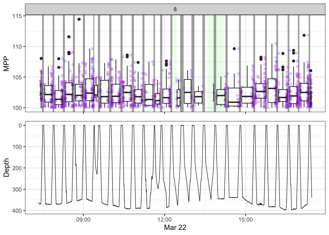

[[9]]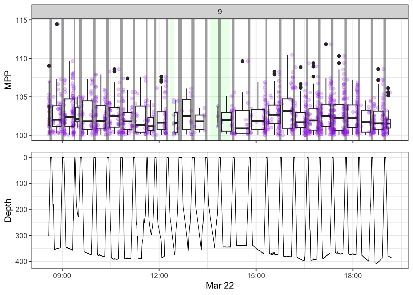

[[10]]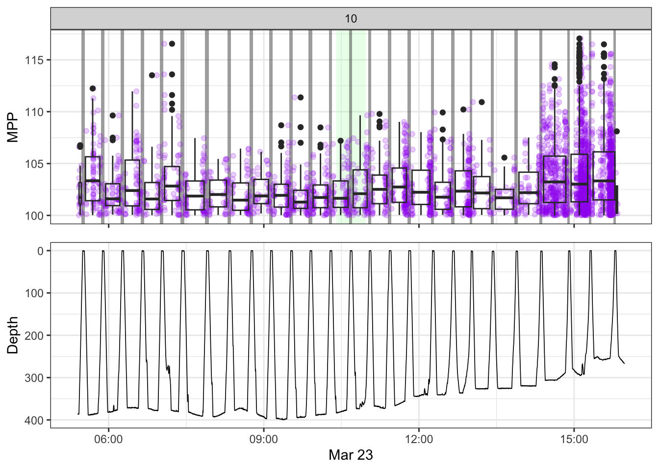

[[11]]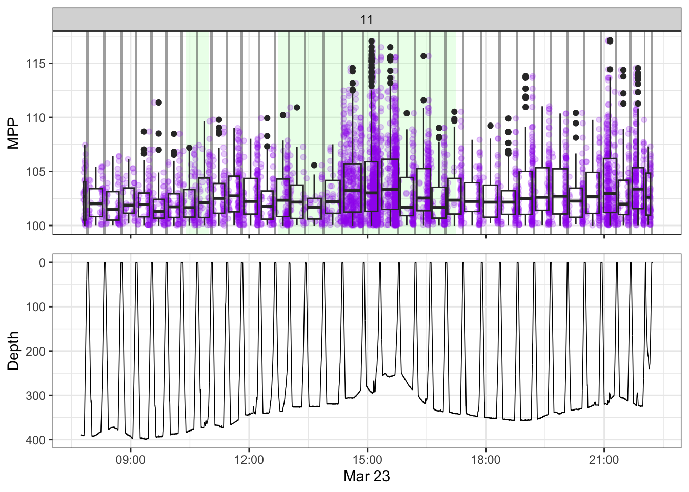

[[12]]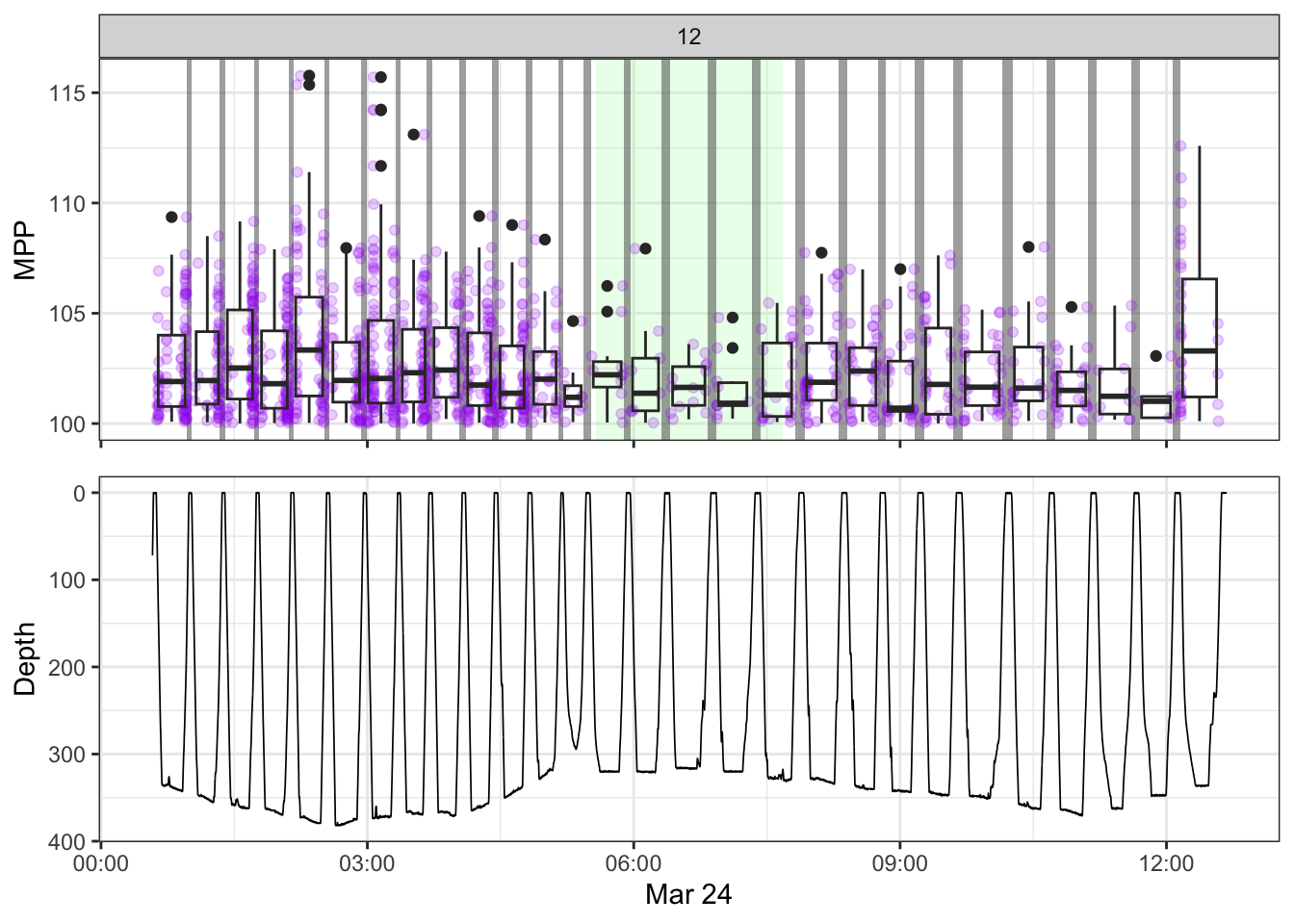

[[13]]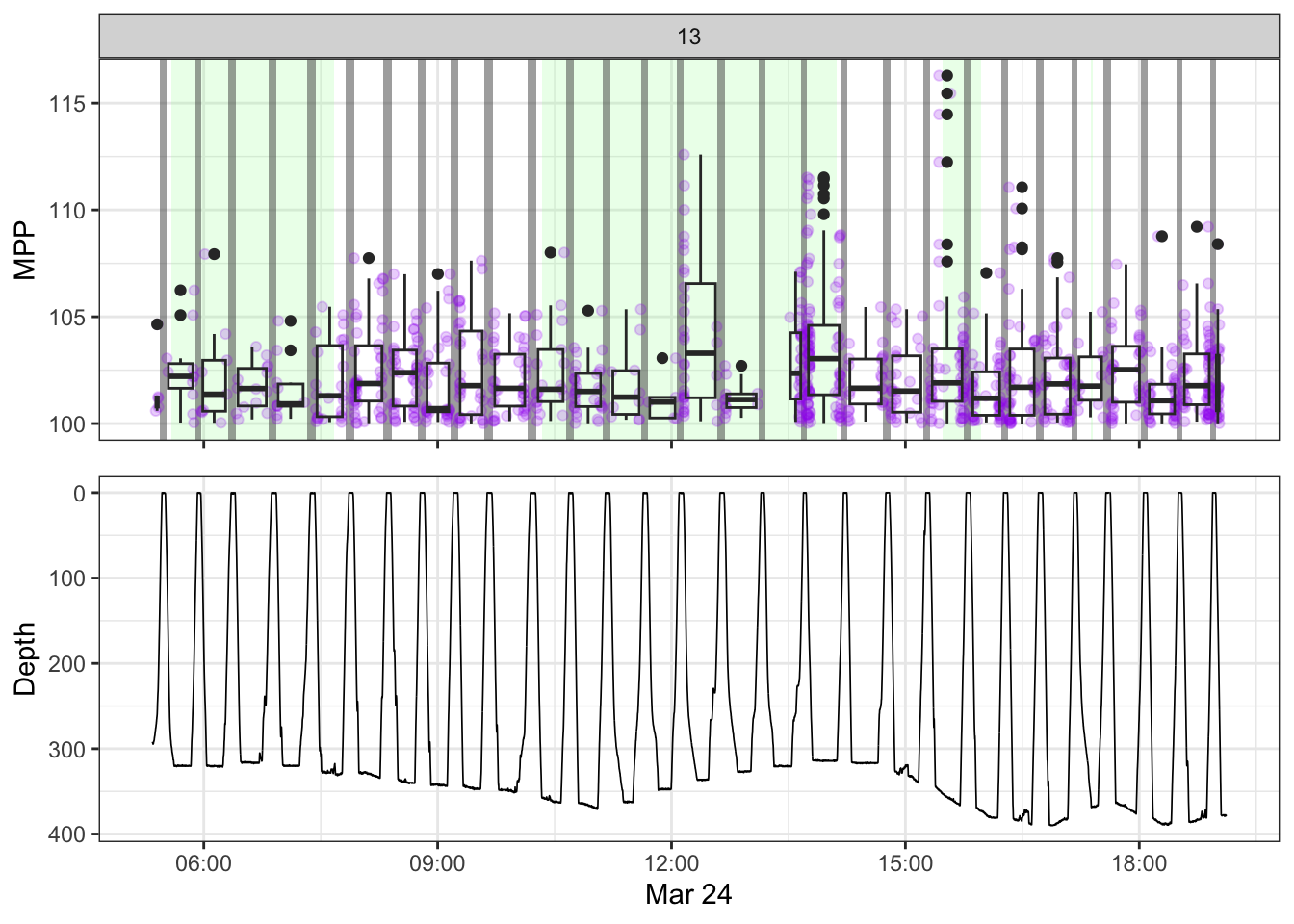

[[14]]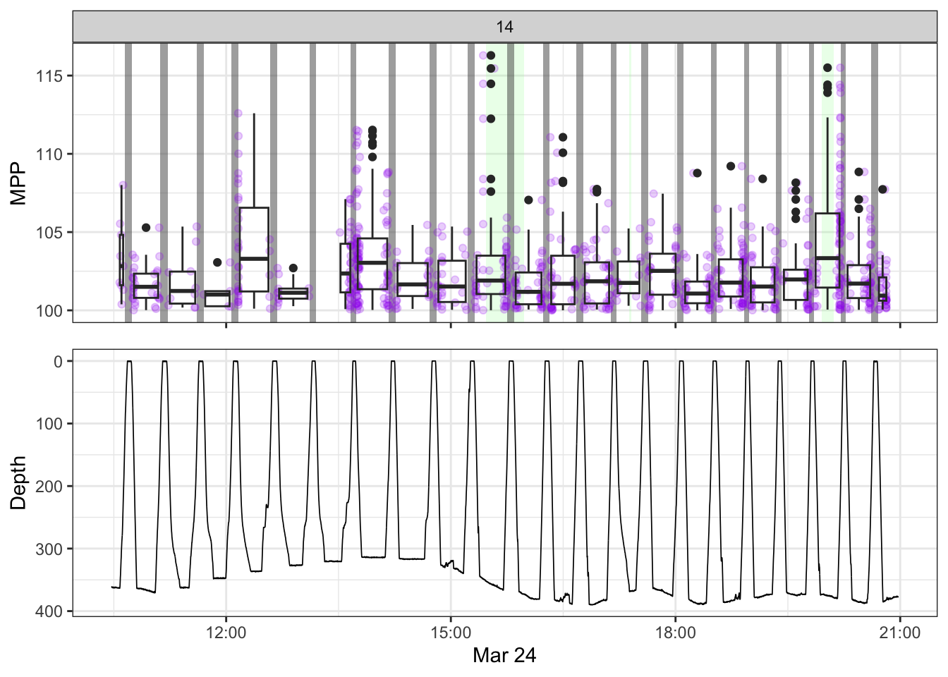

[[15]]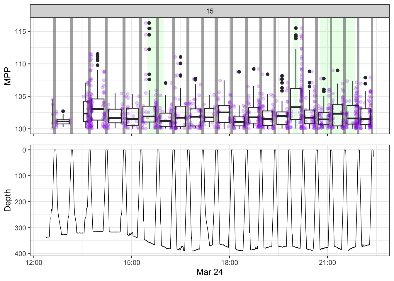

[[16]]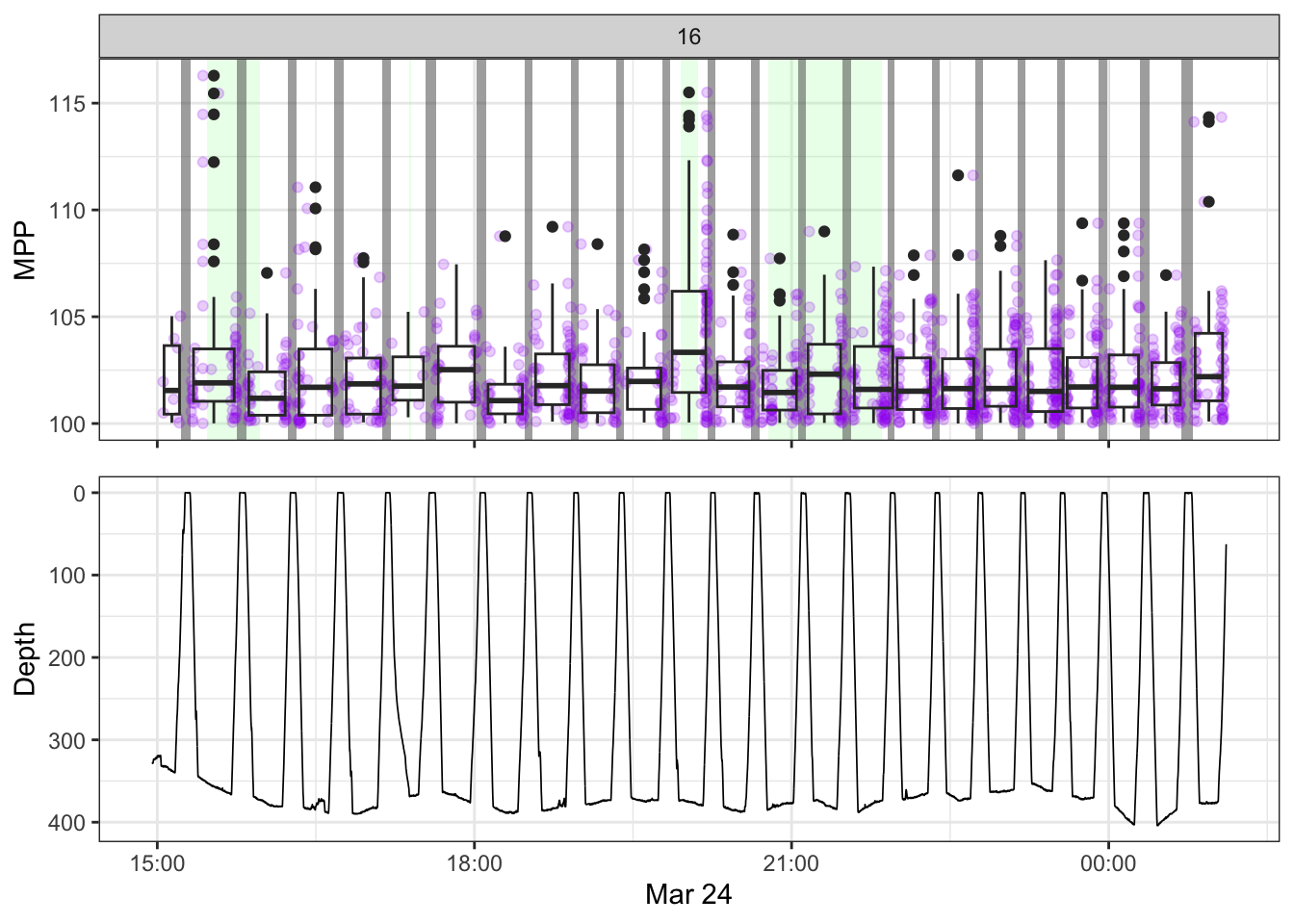

[[17]]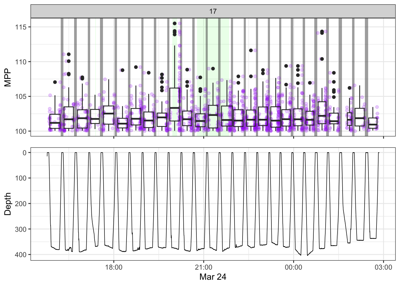

[[18]]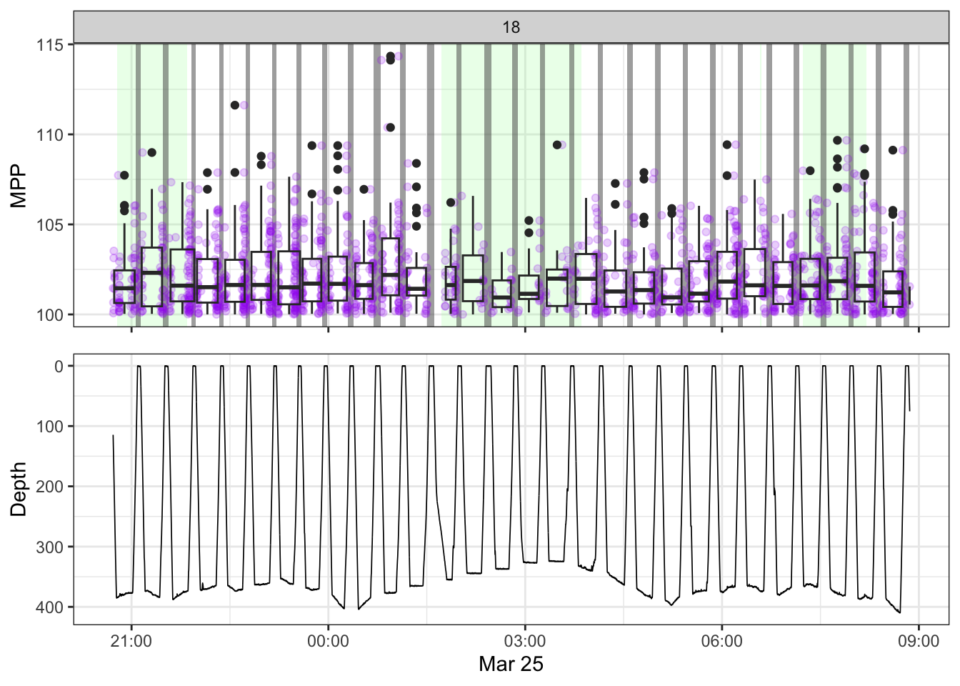

[[19]]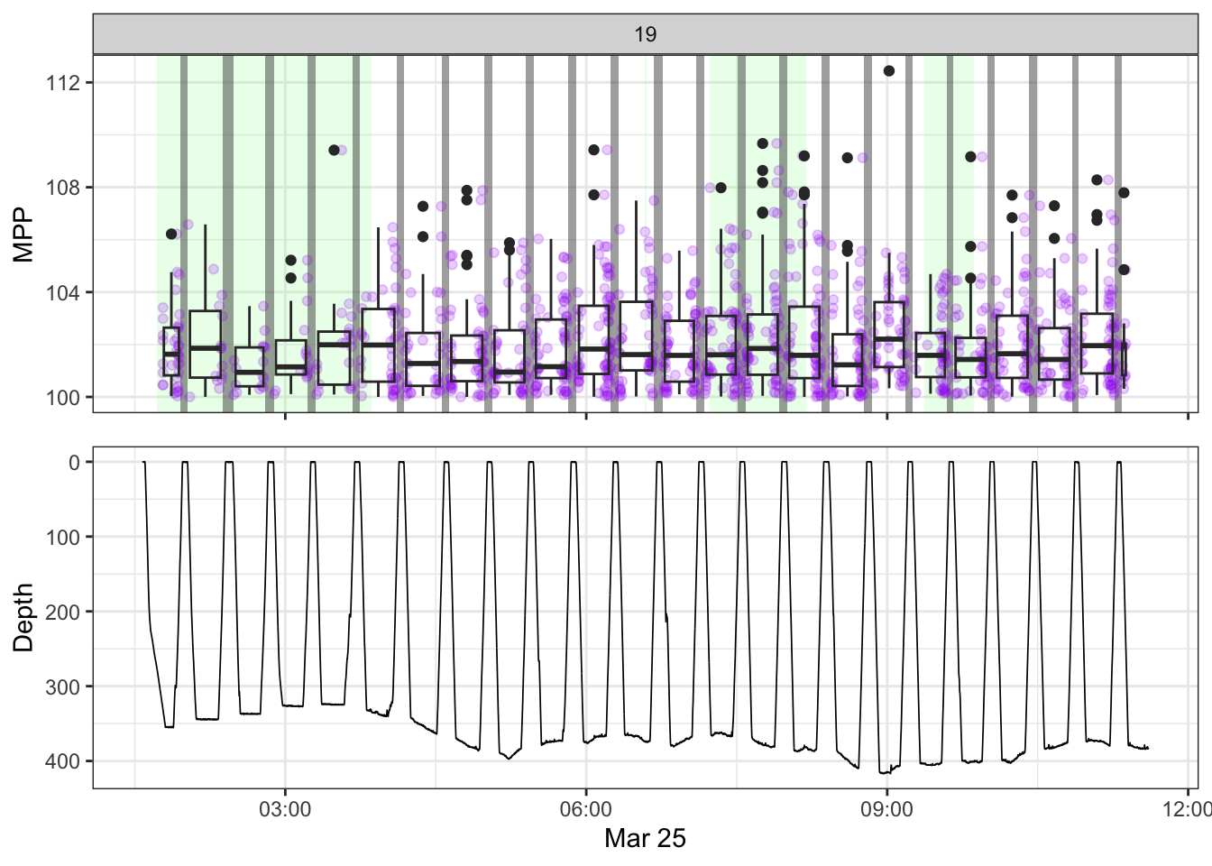

[[20]]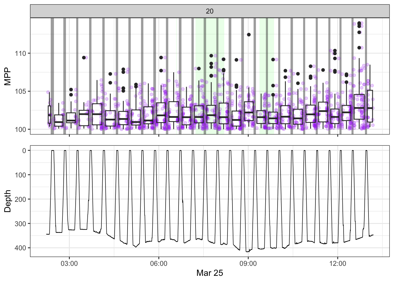

[[21]]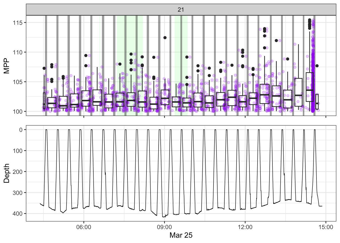

[[22]]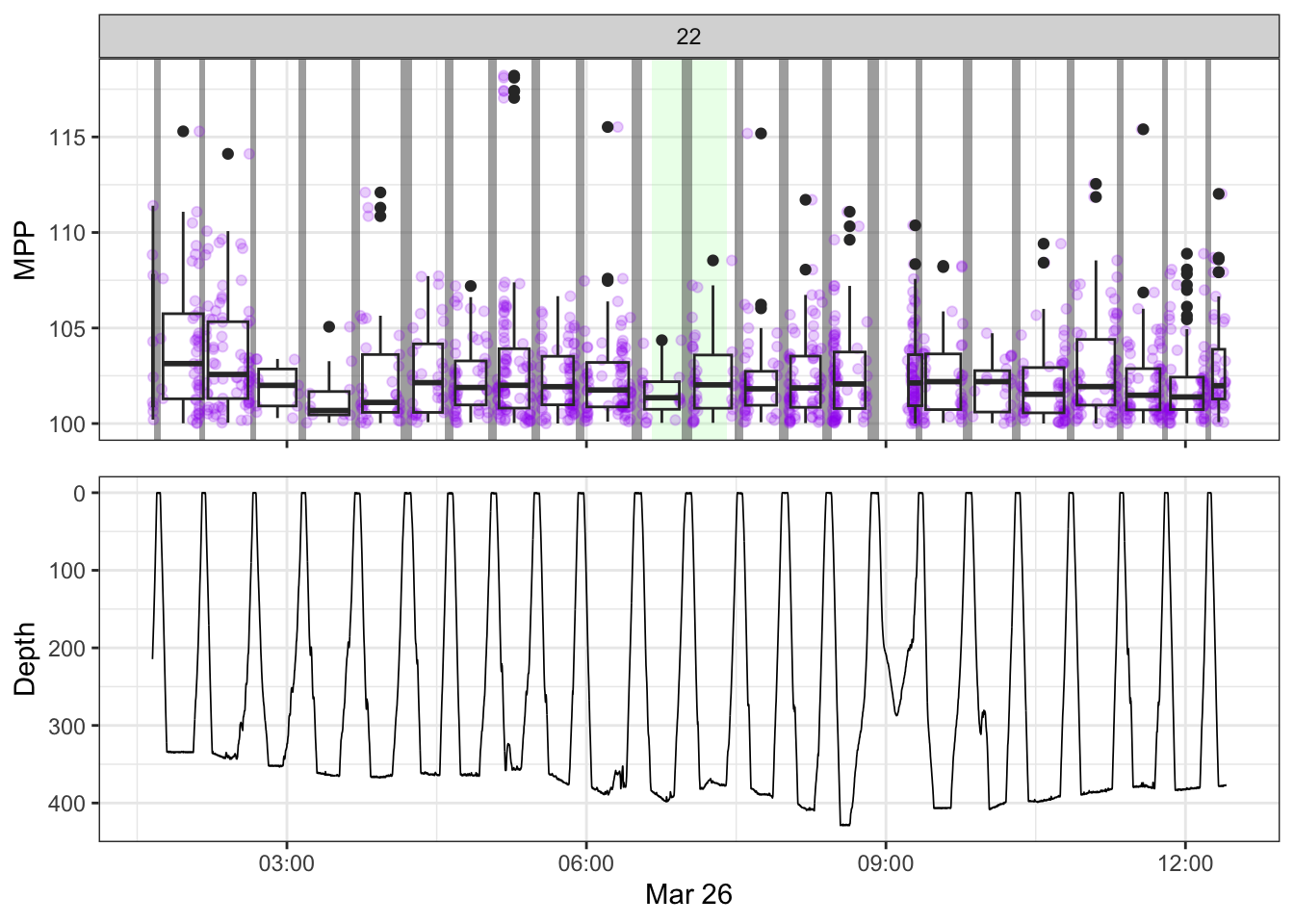

[[23]]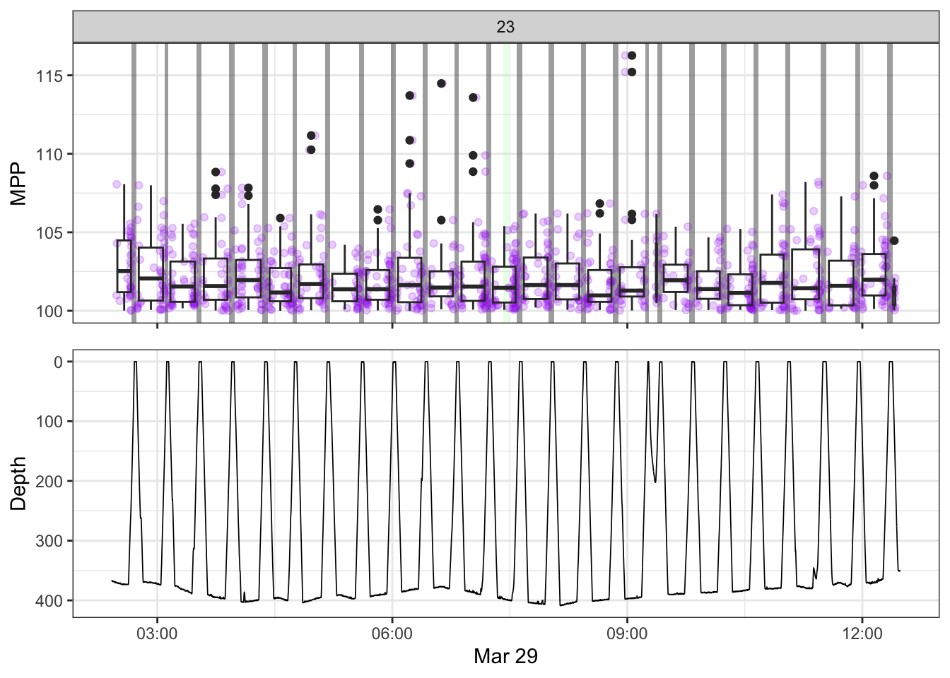

[[24]]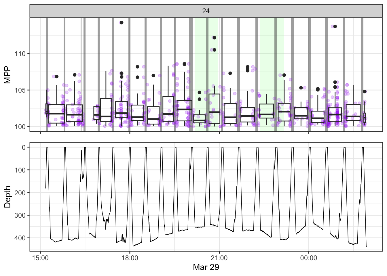

[[25]]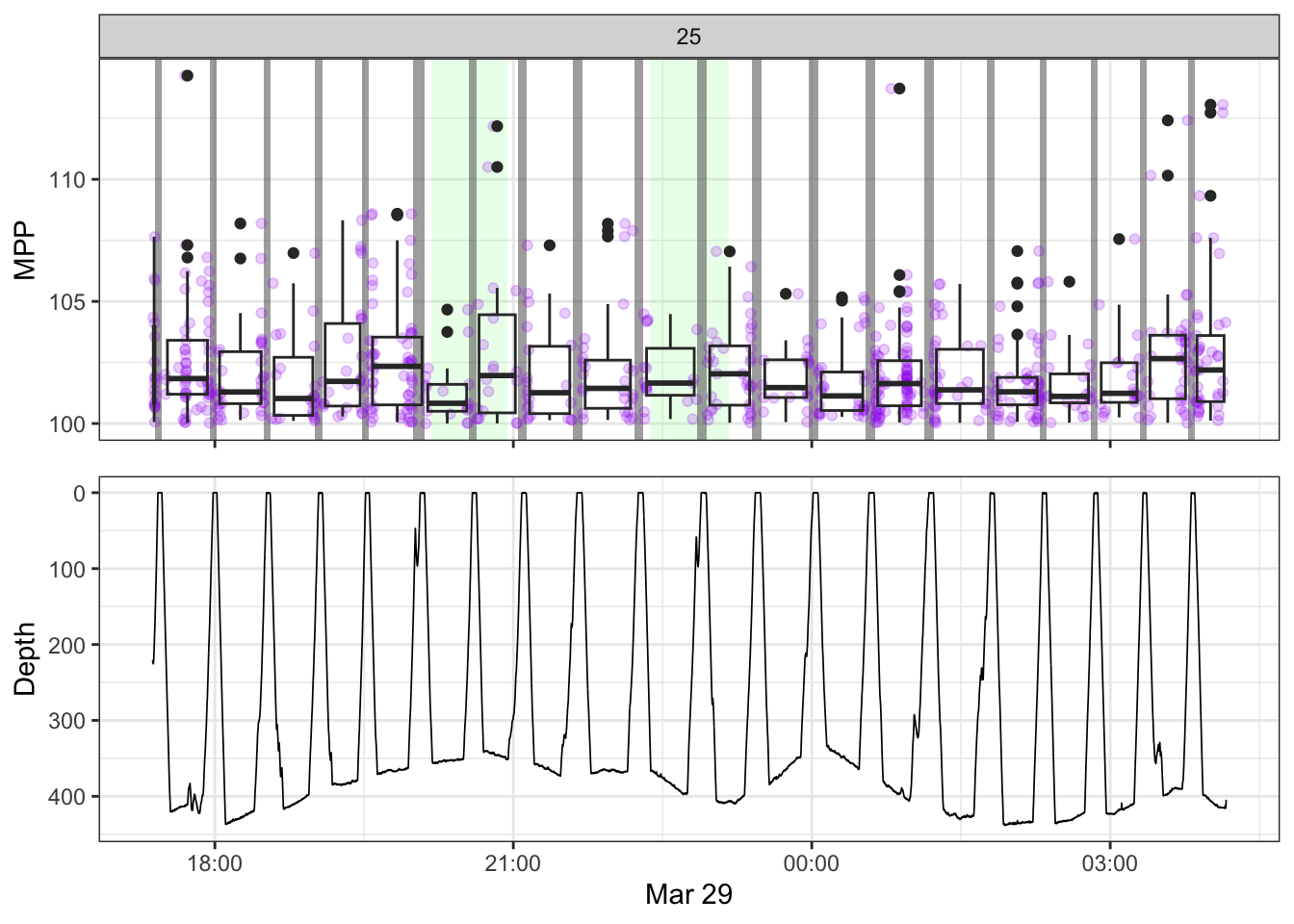

[[26]]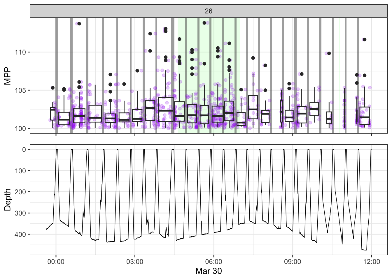

[[27]]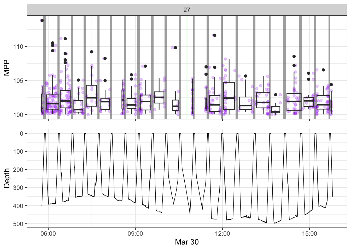

[[28]]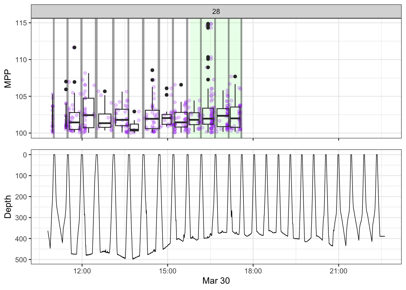

#save the plots to the outputs folder
# map(1:length(bout_plots),
#     ~ggsave(paste0("output/bout_plots/comb_bouts/comb_bout_v3_", .x, ".png"),
#             bout_plots[[.x]],
#             width = 10,
#             height = 6,
#             units = "in"
#     ))