library(aniMotum)
library(tidyverse)
library(terra)
library(tidyterra)

theme_set(theme_bw())Broad scale
Using the aniMotum package as a way to fit a continuous HMM to the seal GPS data.
Loading in our GPS data and formatting it to work with aniMotum:
track <- read_csv(here::here("data/seal_locations.csv"),
                  show_col_types = FALSE) %>%
  mutate(lc = c("G"),
         id = c("H391")) %>%
  format_data(date = "Date_es", coord = c("Longitude", "Latitude")) %>%
  as.data.frame()
Load in acoustic data and aggregate it at 6-hour scale
source(here::here("R/broad_funcs.R"))

#read in the general acoustic data
acou <- read_csv(here::here("data/detections.csv"),
                 show_col_types = FALSE) %>%
  mutate(start = as.POSIXct(start, tz = "US/Pacific"),
         end = as.POSIXct(end, tz = "US/Pacific"))

#read in sperm whale data
sw_valid <- read_csv(here::here("data/SWCombBouts_Validated.csv"),
                     show_col_types = FALSE) %>%
  mutate(start= as.POSIXct(start, tz = "US/Pacific"),
         end = as.POSIXct(end, tz = "US/Pacific")) %>%
  select(-notes)

window_hr <- 6

acou_agg_valid <- tibble(date = seq(first(track$date),
                                    last(track$date),
                                    by = window_hr * 3600)) %>%
  mutate(date2 = date - window_hr * 3600,
         SW = map_dbl(date, \(d) sum_odon_exposure(data = sw_valid, d)),
         SW_lag = lag(SW),
         SW_lead = lead(SW),
         SW_std = (SW - mean(SW)) / sd(SW),
         id = "H391")
Trim spatial, acoustic data to audio coverage
track <- filter(track, date < last(acou$end))
acou_agg_valid <- filter(acou_agg_valid, date < last(acou$end))
Fit model
fit <- fit_ssm(track,
               vmax = 3, #max travel rate
               model = "mp", #fits correlated random walk
               time.step = select(acou_agg_valid, id, date), #6 hour steps
               control = ssm_control(verbose = 0),
               env_formula = ~ SW,
env_data = select(acou_agg_valid, id, date, SW))fit$ssm$H391$par Estimate Std. Error
rho_p 0.32277319 0.16510114
sigma_x 0.44887963 0.05524379
sigma_y 0.70641209 0.06402851
rho_o 0.03194255 0.34306525
tau_x 10.81930842 1.61139800
tau_y 6.30797525 1.49256029
sigma_g 0.01965093 0.13165105
beta -0.16588193 0.09263092est <- fit$ssm$H391$par["beta", 1]
se <- fit$ssm$H391$par["beta", 2]
pnorm(est, mean = 0, sd = se, lower.tail = TRUE)[1] 0.03666401p <- plot(fit, type = 3)$H391
p +
geom_point(aes(date, SW / max(SW)), acou_agg_valid) +
scale_y_continuous(sec.axis = sec_axis(~ . * max(acou_agg_valid$SW), name = "SW (hours)"))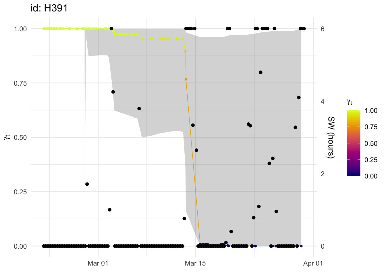
ggplot(fit$ssm[[1]]$predicted) +
  geom_sf(aes(color = g)) +
  scale_color_gradient2(midpoint = 0.5, limits = c(0, 1))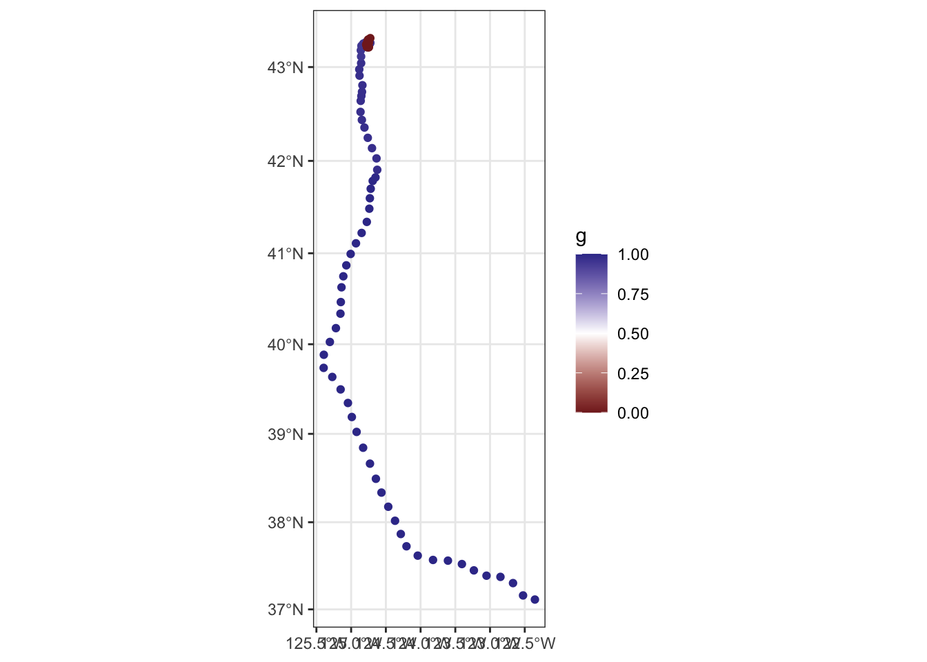
Alternative hypotheses:
1. Luck
Maybe sperm whales and elephant seals both just happened to converge on the patch. If that’s true, then adding a 6 hour lag time or lead time to the model should have similar results.
fit_lead <- fit_ssm(track,
               vmax = 3, #max travel rate
               model = "mp", #fits correlated random walk
               time.step = select(acou_agg_valid, id, date), #12 hour steps
               control = ssm_control(verbose = 0),
               env_formula = ~ SW_lead,
               env_data = acou_agg_valid)
#get lead results
fit_lead$ssm$H391$par Estimate Std. Error
rho_p 0.19919144 0.15905051
sigma_x 0.44423703 0.06657623
sigma_y 0.73359026 0.06321704
rho_o 0.46684533 0.38495589
tau_x 10.23949289 2.01835536
tau_y 4.76564219 1.10122452
sigma_g 0.07987423 0.02810979
beta 0.01232952 0.02845206est_lead <- fit_lead$ssm$H391$par["beta", 1]
se_lead <- fit_lead$ssm$H391$par["beta", 2]
pnorm(est_lead, mean = 0, sd = se_lead, lower.tail = TRUE)[1] 0.6676174fit_lag <- fit_ssm(track,
vmax = 3, #max travel rate
model = "mp", #fits correlated random walk
time.step = select(acou_agg_valid, id, date), #12 hour steps
control = ssm_control(verbose = 0),
env_formula = ~ SW_lag,
env_data = acou_agg_valid)#get lag results
fit_lag$ssm$H391$par Estimate Std. Error
rho_p 0.196700461 0.16587999
sigma_x 0.449972262 0.06474538
sigma_y 0.728503532 0.06234476
rho_o 0.473373512 0.38979437
tau_x 10.714605611 1.98798909
tau_y 4.806354992 1.13613339
sigma_g 0.079656952 0.02661704
beta 0.004146674 0.02625133est_lag <- fit_lag$ssm$H391$par["beta", 1]
se_lag <- fit_lag$ssm$H391$par["beta", 2]
pnorm(est_lag, mean = 0, sd = se_lag, lower.tail = TRUE)[1] 0.5627561A model fitted to the lag/lead values are not at all significant (.5-.6 one-tailed p-test), while the model fitted to the actual values is (0.03, 1 tailed p test).
2. Memory
Maybe H391 has been to that patch before and knew that there was good food there, and she didn’t actually use the sperm whale cue at all.
We don’t know what she does every year, but we do know that for her two other instrumented trips, she traveled offshore - so this isn’t just “her spot.”
#plotting her previous trips
library(ggOceanMaps)
ggOceanMaps: Using /Users/allisonpayne/Local
Documents/Github/Manuscripts/eavesdropping/data/ as data download
folder. This folder is customly defined and does not require
downloading the detailed map data again.library(terra)
library(tidyterra)
theme_set(theme_bw())
pb25 <- read_csv(here::here("data/seal_locations.csv"),
show_col_types = FALSE) %>%
rename(Date = Date_es) %>%
mutate(trip = "PB") %>%
vect(geom = c("Longitude", "Latitude"),
crs = "epsg:4326")
pb_track <- as.lines(pb25)
pm25 <- read_csv(here::here("data/MoreDeployments/H391-PM2025/265936-Locations.csv"),
show_col_types = FALSE) %>%
mutate(trip = "PM") %>%
select(Date, Latitude, Longitude, trip) %>%
vect(geom = c("Longitude", "Latitude"),
crs = "epsg:4326")
pm_track <- as.lines(pm25)
rod <- read_csv(here::here("data/MoreDeployments/H391-RoD/2023228_240257_aniMotum_crw_RSB.csv"),
show_col_types = FALSE) %>%
rename(Date = date,
Longitude = lon,
Latitude = lat) %>%
mutate(trip = "ROD") %>%
select(Date, Latitude, Longitude, trip) %>%
vect(geom = c("Longitude", "Latitude"),
crs = "epsg:4326")New names:
• `` -> `...1`rod_track <- as.lines(rod)
basemap(limits = c(-163, -121, 36.5, 51),
bathymetry = TRUE,
bathy.style = "rcb") +
geom_spatvector(data = pm_track, color = "lightblue", linewidth = 1) +
geom_spatvector(data = rod_track, color = "lightskyblue", linewidth = 1) +
geom_spatvector(data = pb_track, color = "gold", linewidth = 1) +
xlab("Longitude") +
ylab("Latitude") +
theme(legend.position = "none")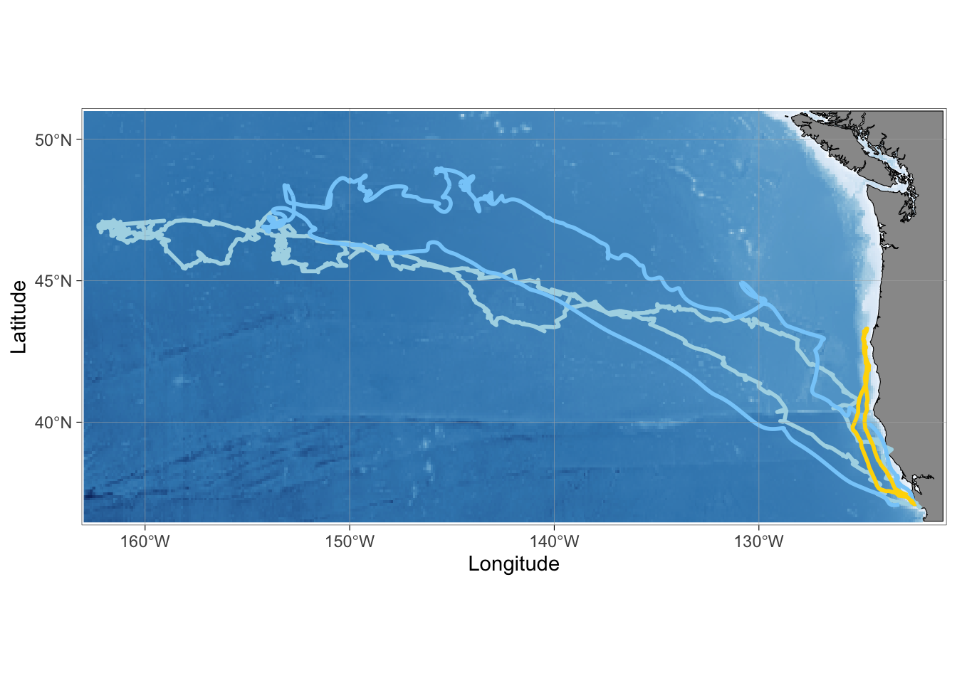
Both of the other deployements were longer trips, but many seals do go offshore on the shorter trips as well. The trip with acoustic recordings is plotted in gold.
3. Other environmental cues
Maybe the seal wasn’t using sperm whales at all, but their calls happened to coincide with another environmental cue, like SST, temp at depth, or FTLE. We could use the tag’s temperature sensor and FTLE measurements to fit our same SSM with oceanographic covariates instead of sperm whale presence and see if the fit is better or worse than with SW.
Let’s try it with average mixed layer temperature, as measured by the tag.
#mixed layer temperature - using average MLT and minimum temperature from this file
mlt <- read_csv(here::here("data/23A1302/out-MixLayer.csv"))
Rows: 236 Columns: 21
── Column specification ────────────────────────────────────────────────────────
Delimiter: ","
chr (4): DeployID, Source, Instr, Date
dbl (14): Ptt, DepthSensor, Hours, PerCentMLTime, MLTave, MLTmin, MLTmax, ML...
lgl (3): LocationQuality, Latitude, Longitude
ℹ Use `spec()` to retrieve the full column specification for this data.
ℹ Specify the column types or set `show_col_types = FALSE` to quiet this message.mlt <- mlt %>%
mutate(date = as.POSIXct(Date,
format = "%H:%M:%S %d-%b-%Y",
tz = "UTC"),
id = "H391") %>%
filter(date < last(acou$end))
# There's one clear outlier in MLT temperature, remove it and interpolate
outlier_idx <- which(mlt$MLTave > 14)
mlt$MLTave[outlier_idx] <- mean(mlt$MLTave[outlier_idx + c(-1, 1)])
mlt$MLTave_std <- (mlt$MLTave - mean(mlt$MLTave)) / sd(mlt$MLTave)fit_sst <- fit_ssm(track,
vmax = 3, #max travel rate
model = "mp", #fits correlated random walk
time.step = select(mlt, id, date), #6 hour steps
env_formula = ~ MLTave_std,
env_data = select(mlt, id, date, MLTave_std),
control = ssm_control(verbose = 0),
)fit_sst$ssm$H391$par Estimate Std. Error
rho_p -0.002985741 0.17545804
sigma_x 0.527465504 0.09355485
sigma_y 0.754052317 0.06994183
rho_o 0.850990319 0.27630706
tau_x 10.382082604 2.39301435
tau_y 5.610716668 1.64725748
sigma_g 0.063225415 0.01963316
beta 0.008299704 0.01812582est <- fit_sst$ssm$H391$par["beta", 1]
se <- fit_sst$ssm$H391$par["beta", 2]
pnorm(est, mean = 0, sd = se, lower.tail = TRUE)[1] 0.6764857p <- plot(fit_sst, type = 3)$H391
p +
geom_point(aes(date, MLTave / max(MLTave)), mlt) +
scale_y_continuous(sec.axis = sec_axis(~ . * max(mlt$MLTave), name = "MLT (degC)"))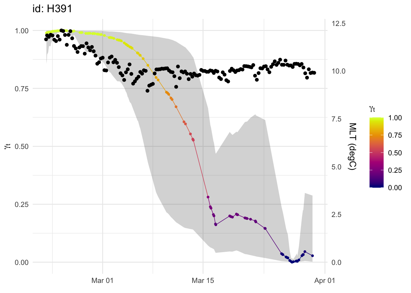
The mixed layer average temperature model isn’t significant. Check the fit of this model compared to the SW model:
fit$ssm$H391$AICc[1] 1374.708fit_sst$ssm$H391$AICc[1] 1409.877SW model is a better fit.
Next step: the fine scale.
We will fit a hidden markov model to the seal’s diving behavior and allow the properties of the sperm whale clicks (received level and peak frequency, both associated with how far away the whales are) to influence her transition probabilities.